What does magnetometer measure ?

1- Introduction :
The magnetometer instrument records the overall magnitude of the field in each point. The magnitude distribution map could be achieved by means of a proper design of the network of a specific region. The magnitude of the field has direct relation with the magnetic characteristics of the rock, which is related to the grade of the magnetic mineral. This exactly stands for the popularity of magnetometering method in mineral deposit explorations. That is because the magnetic mineral has a leading role, different from the beginning stages of the magma subtraction, in its penetration and formation of ultramafic rocks. That would continue up to the last stages of the hydrothermal and injection of the remaining metallic liquids at the magma reservoir into the surrounding rocks and formation of the metallic minerals. Gradually, the magnetic rocks at the surface of the earth face vicissitude and weathering and this would cause them lose their magnetic characteristic and change into the iron soil (as known to mine owners).

The aim of magnetometering measurement is surveying intact magnetic mineral deposit status in deeper regions. This fact clearly justifies the accomplishment expenses of studies as such. The above-mentioned points are also valid for Aliabad iron deposit. Diffused oxidized outcrops were observed wherein their qualitative carat and geometrical status in the intended depth were surveyed and their model was obtained in this study. Through these models, we could obtain a general perspective from the total reservoir volume under investigation.

In this report, we also applied the software such as Excel, Geosoft, Surfer, IGRF internet program and free software of Mr. Cooper, Withwatersend University in South Africa.

2- The Region under Investigation
Ore mineral geophysical operations region is distinct on the 1:100000 of Tarom geology map (map1). The execution procedure of measuring points was defined according to surface outcrop and extracted trenches.

2.1. Geographical condition and access to Mineral deposit :
This region is situated at km 3 east of Sorkhedizaj village, 40 km far from northeast of Zanjan. There are two main ways to access the region. One way is that passing about 22 kms on Zanjan-Tehran road, you reach a side road leading to Sorkhedizaj and Morvariyeh. Having passed about 10 kms of this side road, you arrive at Morvariyeh and it is about 4 km from Morvariyeh to the exploratory region. Another way is to arrive at the region is an asphalt road from ZanjanTehran road that after 8 kms it reaches the southeast of region.

2.2. Weather condition
Concerning weather, mineral deposit region has cold winters and mild summers. The average temperature in winters is about -28 °C and in summers +30 °C. This region has foggy, snowy and stormy weather, especially in winters, and since it is close to Tarom Mountains and has torrent air, sometimes snow and blizzard prevent any kind of mineral or exploitation activities. The herbaceous covering of the region is sparse and generally lacks wild tall bushes or trees. However, south parts of the region, which encompass alluvial plains, include farms.

2.3. Region General Geology
Aliabad exploitation region is situated in 1/250000 Map of Zanjan and 1/100000 map of Tarom (figure 1). According to constructive sedimentary main fields of Iran, it is situated in the central field (Aghanabati 2004) and AlborzeAzerbayejan geology zone. The oldest stone unit of Tarom plate includes calcic stones as old as Devonian that is scarcely outcrop in northeast plate.

2.4. The Exploitation Region Geology :
An extensive part of exploitation region consists of Tertiary volcanic and penetrative stones. The previously mentioned volcanic stones with general eastwest extension developed from south-east to north-west and there are some kinds of penetrative piles with high compound amounts of Monzonite, quartz monzonite and Monzodiorite with Upper Eocen age inside them (figure 1).

On the east of exploitation region and near Sorkhehdizaj iron mine, there are quartz monzonite – monzonite apophysis like bumps on farms in which iron veins were observed, either in their contacts or inside them (Figure 2).

2.5. The method of marking the points and measuring data
In the first exploration region, a big outcrop of iron was observable in form of a vein. To start the investigations, we decided to install some profiles perpendicular to outcrop. According to this outcrop and its surrounding, measured by 1510 stations, the distance between profiles was defined to be 30 meters and between points, 10 meters in sequence and in north-south direction (map2). The outset and the end of any profile was designed in such a way that the magnetic field limit along the profile started from a zonal base limit and passing the abnormality limit it came back to the base limit at the end of the profile. This base limit was obtained according to the global magnetic field and a number of measurings before implementing campestral operations in the investigations of the region.

3- Magnetometer instrument
The device used in this report was magnetometer proton WZ-1/3, made in China, with the following technical specifications:

Main Features:

- Geomagnetic field and normal gradient of geomagnetic field sounding (horizontal gradient component of geomagnetic field or vertical gradient component of geomagnetic field, special sonde and support are needed);

- Applicable in field survey or base station measurement;

- GPS carries out real-time positioning so that operator can be navigated to the next preset measuring point;

- Built-in clock can be set by GPS time synchronization automatically;
- Measuring result of each point consists of position information such as latitude, longitude, elevation and time. User can perform time measuring and storing actions as well;

- Designed with a back rack, magnetometer, GPS, sonde, GPS antenna and battery, operation is easily fulfilled by one person;

- Integration of clock: record time is stored together with the data measured at that time.

- Large display, English interface to display magnetic curves automatically and easy in operation.

- Backlight LCD screen can be used at night.

- User-friendly keyboard can be used by both hands.

- Automatically or manually tuned.

- Portable, one person can finish all the fieldworks, for the system is designed with gallus.

- RS-232C port.

Technical Specifications:

- Measurement range: 20,000nT~100,000nT

- Measurement precision: 1nT

- Resolving power: 0.1nT

- Allowed gradient: <=5000nT/m

- GPS positioning accuracy: <2.5m CEP

- Data stored: 50,000, power-off protected

- LCD display screen: 240x128

- Keyboard: 22 keys

- Interface: RS-232C standard serial port

- Power supply: External rechargeable batteries, 14.5V/3Ah, or external power supply

- Dimension of mainframe : 230mmx155mmx65mm

- Weight of mainframe: 2.2kg (include batteries)

- Dimension of sonde: ∅75mmx155mm

- Weight of sonde: 0.8kg

- Working temperature: -10℃ ~+50℃ (Environment temperature)

4- Data processing

4.1. Eliminating daily effect
In this stage, the earth magnetic field temporal effects, related to spatial sources, were eliminated by a station magnetometer. This device should be located at less than 50 Km far from the working region. Through a primitive survey in the region, we found that the anomalies’ scope was so extensive and there was no need to record the temporal changes, and accordingly we gave up installing the base station

4.2. Eliminating IGRF effect
After eliminating the field temporal changes, the field related to earth core, upper mantle and deep parts of crust that were not considerably valuable in mineral exploration, were subtracted from data. This was done by IGRF program. The region longitude and latitude, height and measuring time were the program input and earth field slope, angle of deviation and field factors measures were the output. The field features are illustrated in table1 in the latitude of 1980 meters and by using updated IGRF.

4.3. Eliminating the noise :
Considering the magnetic nature of region magnetic sources, plenty of noises could be created in the data resulted from combining region stone with this mineral. However, the afore-mentioned region data were so valid and appropriate and its noise amount was so limited. Non-linear filters also eliminated these limited amounts.

After applying such processes, the region anomaly field total magnitude map (TMA), that is also called residual map was prepared. This map became the basis of further analysis.

5- Analyzing and Interpreting the Data :
The source of the earth magnetic field is located at the core. The magnitude of this field, as mentioned earlier, is about 30000 Gama at the equator and about 60000 Gama at the poles. This means that it reduces from poles to equator and it is mostly like a bi-polar field. This field causes a secondary field in the crust rocks that is the magnetic anomaly (Figure 3). In this regard, two types of qualitative- quantitative analysis have been ever used which will be further explained in the following section.

Map 3: The magnitude of Anomaly Field

5.1. Qualitative interpretation:
In this phase, the qualitative characteristics of the anomalies in the region under investigation were studied. These characteristics would include the magnitude of the field, context, sidelong expansion, type of the source (Dike, contact, or etc.) remnants magnet and the remaining magnetism in the rocks from the Paleomagnetism era. Extracting all of these items from the maps depends on the experience of the interpreter and analyst of data nature and physics and this stage is the basis of further ones. It is expected that in the stage of qualitative interpreting, the geometrical and physical features of known existing sources and to some extend mineral deposit model and its relation with region geology would be achieved.

Note : the physical nature of earth magnetic field in the northern hemisphere causes an anomaly surveying from south to north. This, in the first step reflects its positive pole (red) and then the negative pole (blue). Figure7.

In Map 3, the map of region anomaly total magnitude was considered. The approximate outcrop of magnetic vein was shown on the map. Without any kind of analysis, one would understand that the region magnetic map has more potentials besides what is revealed on the map.

5.1.1. The map of reduction to northern magnetic pole:
As mentioned before, the nature of magnetic anomalies was bi-polar and their creative source was situated nearly between these two poles. This phenomenon is one of the complexity reasons of magnetic maps analysis. To solve this problem, the filter of reduction to RTP pole transferred the magnetic anomalies to northern pole through mathematical methods. The magnetic vector entered the earth vertically in the north magnetic pole that on one hand caused an increase in the North Pole and was situated exactly above its source and on the other hand caused a decrease in the south pole that migrated to the outskirt of the anomaly (graph 4). In this way, the complexities of the anomaly overall magnitude decreased to some extent and the magnetic sources superposed the positive poles (the red color in the graphs of this report). It should be noted that the basic hypothesis of this filter was that magnetic field of the source mass was in the same direction as the magnetic field of the earth. However, where the magnetite exists, due to the powerful respond of the mass, this hypothesis is not quite valid and should be applied with much more care. Therefore, it is better to use the major map of the field magnitude as the basis for analysis.

Locating the mineralization zones approximately by using the place of the maximum anomaly is another application of this filter (map 4). In this figure, the reduction to pole map is illustrated and the probable areas of magnetite mineralization are represented in dark color. As it is evident in this map, 4 magnetite veins penetrate the area under investigation from east to west. These veins are in some places of high carat and in some others of low carat. Also some faults have cut these veins several times. This is further detailed in the following sections of the report.

5.1.2. Vertical derivative map
The more we move away from the magnetic sources, the more extended the anomalies become. This means that the surface sources have sharp anomalies and the deep ones have softer responses. The vertical derivative transformer is designed in a way that weakens the deep sources and reinforces the surface ones (or the shallow parts of a source). In case there exist scattered sources on the earth surface, this filter produces more noise. Applying this filter to the reduced data to the pole would provide a vivid image of the area’s masses. For the purpose of troubleshooting the data was applied to the altitude of 5 meters above the upward continuation of measurement level and then the vertical filter was applied to it. Much more details of the magnetic veins have been revealed in the vertical derivative map of the reduction to pole (map 5). For example, it was observed that the two upper veins had breaks in some places and the lower one comprised of two other veins. In this map, the oxidation and alteration areas were more vivid, compared to reduction to pole map.

5.1.3. The Faults and Magnetic Joints:
Recognizing the faults and magnetic joints is one of the most important stages of qualitative interpretation and the interpreter can recognize the overall structure of the area and obtain more information for the qualitative interpretation stage. Map no. 6 illustrates the faults and magnetic joints. The main development of the magnetic anomalies and joints was from north west to south east. There was also another joint system that developed from north east to south west which was perpendicular to the other system. The background map is the vertical derivative map achieved from the data reduced to the RTP pole which was explained earlier. Many interpretations can be made from this map which are not included in the scope of this report. However, the condition of the joints indicate that most of anomalies were cut by these joints but it was not possible to state that the mineralization of iron was related to these joints and they were not the best controllers for iron ore. Proving the relationship of mineral formation requires more extended maps of the area under investigation. This issue will be used extensively in quantitative analysis. Moreover, since the area was covered with farm soil, it was not possible to recognize the small faults of the area. Therefore, theses magnetic joints could help in designing the mineral extraction. The joints that could make changes in the anomalies can be called faults and they have been approached the same in joints maps. Most of the existing joints can be called faults. Aggregation of a lot of joints in the anomalies of south west caused the mineral to break and this made it impossible to observe any homogenous sources in this area. On the other hand, the anomalies in the north were less broken (not cut) and these more homogenous anomalies were noticed to a greater extent from economical point of view

5.1.4. The Upward Continuation Map:
Conversion of the upward continuation, contrary to the vertical derivative was designed to weaken the surface anomalies and strengthen the anomalies of deep sources (map 7). As a result, by applying this filter we could gain more qualitative information about the depth of the source (metallic masses) development. Contrary to the common belief that this filter would provide us with sections of the mineral in different depths, it would never give any quantitative information about the depth of source development. In addition, it would not define the depth at which the mineral would finish.

As you can see in map number 7, the development of the anomaly at the center of the area from west to east was uninterrupted which illustrates the fact that the mentioned source was unique and has changed to this form by the movements of the faults. In addition, the effect of the surface anomalies has reduced and disappeared. As it was mentioned before, the upward Continuation of data with different heights, the depth of the mineral would not be defined and just the relative condition of the existing sources would be considered from the depth viewpoint. The maps of upward continuation defined that the anomalies of area in the north were weaker in the basis of depth and the more the height increased the more the depth decreased. On the contrary, the anomalies of the south showed a consistency in the depth even at the height of 100 meters and were deep enough. As it was discussed in the section concerning the joint this area had lots of faults and the vertical derivative map showed that the south anomaly consisted of two neighboring veins. The upward continuation map indicated that this break was just Page 23 Application Case of WZ-1/3 Proton Magnetometer_Tarom. Tehran, Iran BTSK/W.T.S Limited www.wtsgeo.com Page 24 at the surface and the depth source of the veins near the bend was the same in this place.

5.1.5. The area mass’s borders map:
One of the instruments for qualitative analysis of the data of magnetite measuring is recognizing the borders of the magnetic units of the area. As it was indicated earlier, the magnetite measuring maps are complex in their own respect and the characteristics of anomalies would not be recognized easily. Various methods have been suggested for defining the borders of magnetic masses among which Blakely & Simpson (1986) have been used here which was based upon pseudo gravity and horizontal gradient. This is illustrated in map number 8. For comparing the base map with the borders’ one the anomaly overall magnitude map was considered so that it might reflect the anomaly deviation from the source. The surface sources are highlighted in dark points on the map. Connecting the points by drawing a line would define the border of the mineral masses. For defining the priorities, we marked the border of the major veins by bigger points and the minor veins by smaller ones. These areas show the area above the mineral which had outcrop in some places and in most cases has been placed beneath the surface oxidized layers. It should be noted that the borders were defined on the account of a number of presuppositions such as verticality of the mineral edges, inducing charactristic of the field and lower amount of magnetism rocks. However, these presuppositions were not absolutely correct always and therefore these borders were not definite and just represented the approximate edges of the mineral and needed to be incorporated with other information.

5.1.6: The final qualitative analysis map:
Using all the information in this project, a map was developed that highlighted qualitative characteristics of the magnetic ores (map 9). The dimensions of the magnetic masses were marked in black. It is worth mentioning that the above mentioned areas are merely the horizon above the mineral which had been outcrop in some places and buried in some others. The vertical development of these masses is to be applied in the numerical analysis. The relation between these masses, joints and faults of the area are defined clearly. The qualitative analysis map shows that the magnetic vein recorded on the surface of the earth, the track of which was lost in some places, had not developed to south. Rather it had continued from east to west, concealed beneath the surface. Also in the southern areas there existed two magnetic veins, one of which was thick enough and the other was unsatisfactorily thin and discontinuous. For defining the economic issues for the vein, the mineral deposit was divided into two groups of high carat and low carat. The high carat ones were the outcropped magnetic veins and the low carat ones were those concealed beneath the surface of earth. These veins were probably the ultramafic dike rich in the magnetite ore that did not worth anything at all. However, some trenches were suggested in the subsequent steps to confirm this issue. This map has approximately defined the condition of iron mineralization in the area and has provided the interpreters with suitable data so that it might avoid any mistakes in numerical analysis and that would lead to presenting figures and numbers that would contribute to the progress.

5.2. Data quantitative analysis:
Having defined the condition of magnetite masses and crucial areas in terms of mineralization, these areas were studied in details once more and their characteristics such as depth, material and development were defined in quantitative figures. In fact, this chapter represents the results concerning the mineral deposit condition. It should be noted that the numerical analysis has always been subject to uncertainty in geophysics. Moreover, this information can on one hand be crucial in the subsequent decision-makings and on the other hand cause mistakes and deviate the process. This issue is not the goal of this report and is excluded. The point worth noticing is that uncertainty of the results depends on a number of factors, the most important of which include the quality of the data and the physics theory of the issue. Theoretically, this means that there are indefinite sources in the earth that can reproduce the existing anomaly. Selecting a method out of an indefinite collection is quite difficult and requires the knowledge of the interpreter. The best way of overcoming this problem is having complete subordinate knowledge of the area which can be obtained in different ways. The geological information of the area is available while no geophysical data of the area such as magnetization of mineral deposit and the excavation logs are available. This causes problems for carat and deposit qualitative analysis. The magnetic anomaly of Ali Abad followed the simple physical formation and consequently the results were more reliable. Since the anomalies develop in linear formation, the changes happen along the development. Therefore, the L15 and L23 profiles were selected for modeling. L15 profile was known as the representative of Ali Abad overall mineral deposit because it had cut all the mineral deposit. However, since the anomaly of the two neighboring masses in the south of this profile combined with each other, first the L23 profile and then the L15 profile were modeled. Considering the data from the previous section and the ground observations, it was concluded that the dike model could represent the anomalies of the area best.

5.2.1. 2D and D 2 1/ 2 Talvani Modeling:
This modeling has long been used in gravity and magnetometry analysis for its simple nature. The hypothesis in this method is that the extension of the source Iin oibne direction exceeds the other directions and this hypothesis includes nearly every extended source such as dikes, faults etc. in geology. In such structures, we can suppose that the quality of mass remains consistent along the extension (2D sources). To solve the above-mentioned problem, some revisions were applied to this method and so there is no need to higher tensions in one direction than other directions ( D 2 1/2 sources). In this method, we can almost find all (source) model parameters such as quality, depth and geometrical figures (for more explanations refer to relevant articles). The main point is that models were the whole ore zone –that according to existing limitations they are shown homogenous – not just the high carat mineral deposit

A) Profile model L23:
This profile is in south to north direction, situated in the central part of region, and nearly has cut all anomaly zones. Figure 9 shows the gained model of this profile.

This model shows a dike like lens with an average thickness of 10 meters and length of 30 meters. Its magnetism is about 1 in SI that from the viewpoint of mineral is equal to a valuable carat. For more information on mineral deposit zone A refer to figure 9. This reveals the fact that the mineral status has particular complexity and needs more analysis. Nonconformity of the made curve (chromatic) and real curve shows that there are other sources near mineral ore and also interrupts the primary hypotheses such as merely induced field and source 2D interrupted.

B) Profile model L15:
As it is observed this model contains four magnetic veins in region, two of which have outcrop and the other two are hidden. These masses’ thickness is between 1 and 6 meters but they are not definite, as the susceptibility states. However, regarding the difference in thickness of crust between the real and the Page 30 Application Case of WZ-1/3 Proton Magnetometer_Tarom. Tehran, Iran BTSK/W.T.S Limited www.wtsgeo.com modeled one, executing trenches and excavations in the mentioned places was suggested. The magnetite mass located at the south of the profile reflected a slope towards the north while in the model it was towards the south. This phenomenon could be proved or rejected simply by executing the trenches. The resulted magnetism stands for high carat veins. The average magnetism of this profile models is about 2.

6- Conclusion and further suggestions:
The geophysical studies of the area lead into the exploration of two hidden mineral deposits and the pertinent investigations of the geometrical conditions and the carat of the deposits in the previous chapter proved that the magnetite was deep enough and well extended. In addition, it proved to be of good carat from economical viewpoint. The ground observations established the homogenous nature of the mass. These studies mostly depend on the implementation of some core-barreling, trench excavating, and sampling exploration activities from the depth of the mineral deposit. The proper place of these exploration operations are presented in table 2 and are highlighted on map number 10. Unless the exploration results show higher degrees of carat, there will be remodeling so that it might lead into new results. In addition to the suggested points, some others would also be excavated or exploited based on the expertise of mining engineers, area’s anomalies and conditions. Having taken the models for granted and with respect to the above-mentioned facts along with the experience of interpreters and conditions of the magnetic field, it is predicted that the overall anomalies of the zone do not exceed 300,000 tones of mineral. This estimated figure represents the overall magnetite in the area, the whole of which is definitely not extractable. Moreover, the real carat of the mineral would not be measured precisely, while the results prove the purity of more than %45. Presenting more information is beyond the scope of this research and requires further investigations and studies. Due to shallow mineral deposits of the area, excavating trenches is preferred to core barreling and this would save both time and cost.

Table 2: the suggested points for excavation

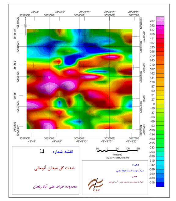
7- The Primary Investigations for Identifying Prospective Areas in the Northwest of the area:
As employer had ordered, at km 3 Northwest of the area, 8 profiles were executed for the purpose of primary recognition and identification. Six of them were with 100 meters of distance from each other and the other 2, as the medial profiles, were with 50 meters of distance from each other (map 11).

The map of the overall field anomaly and reduction to the pole of this area is highlighted in maps 12 and 13. The anomalies of the area extended from east to west and did not seem to be powerful anomalies from magnitude viewpoint. Most of the recorded anomalies of the area were in mass form. These anomalies were usually formed by ultramafic igneous masses with high percentage of iron.

In other regions, there are some other anomalies with smaller dimensions but more extensive and dike like type that would belong to magnetic thin veins in the region under investigation. Because of the high potentiality of the region in iron mineralization and the possibility of existing high carat mineral deposits in the mentioned rocks, the anomalies were analyzed and the promising regions were identified for further surveys.

In map number 14, the boundary of masses that contained magnetite is shown. The investigations show that these masses were put in the ultramafic rock Page 39 Application Case of WZ-1/3 Proton Magnetometer_Tarom. Tehran, Iran BTSK/W.T.S Limited www.wtsgeo.com class with high amounts of iron. In the areas that in final analysis map excavating trench was suggested, there probably existed magnetic veins. Because of the far distance between profiles, it was not possible to determine the precise expansion of the zones which contained ore. Finally it is suggested to excavate trenches in the regions defined in map number 15 and in case of good result measuring a magnetometry grid with higher resolution in the mentioned places would be preferred in order to use its results (vertical and horizontal expansion and final models figure) to estimate the reservoir. In table 3 excavation coordinates are shown. Regarding the result weakness from the viewpoint of iron mineralization in this area, the trench is advised to be excavated under the supervision of a geological engineer in the defined areas.

Table3- The suggested excavation points in northwest of the main area