Geophysical Studies of Khorablou Magazine Dam

Preface
In respect to the geo-physical studies in Kharablou region located in Western Azerbaijan Province, these researches have been started by the expert group of Tarh Noandishan Company. The geophysical studies in Kharablou region have been designed and performed with utilization of two different methods.
This part of the report “The Geo-electric studies” elaborates on the designing method and performing the studies and the preliminary geological interpretations resulted from the geo-electrical evidences.

The aim of performing such investigations is as follows:

Regarding these aims, after performing the field and book investigation, the geo-electrical studies have been designed and performed using the Schlumberger within the limit of the subject of research.
The geo-physical investigations using resistivity method generally includes 96 measurements which have been performed with method of vertical electrical sounding (V.E.S) Schlumberger with the maximum 600 m current line length. The profiles include 8 survey lines on the east-west axis (with the soundage distance of around 25 m) or 12 north-south profiles. The results from the primary interpretations of the measurements in the form of apparent resistivity section have demonstrated the apparent resistivity maps. The achieved results have been elaborated on and concluded from in this report.

Section One: General Principles
The electrical surveys are the most various geo-physical methods. This geophysical investigation method is based on the revealing the effects from the surface resulted from electricity transmission into the ground. Using the electrical methods we can measure the potential and electromagnetic fields existing naturally or produced artificially inside the ground. This is possible to do this in various ways achieving various results all of which help us realize a unique matter.
One of the electrical characteristics of earth is the existence of changes in electricity conductivity in the rocks and minerals. This characteristic has made the electrical methods possible. One of the most significant electrical methods is the apparent resistivity method. This method can provide useful underground geological information which usually should be obtained through other expensive geophysical methods. Amongst the applications of the apparent resistivity method is realization of the buried canals, surveying the underground water, ground movement and also studying the Karstic regions, natural and artificial underground caverns.
This method is also suitably used in civil engineering. In such studies the said method is generally used for realization of the alluviums thicknesses, depth of the table water surface, depth of the bedrock, identification of the clay layers in a vast capacity. One of the significant applications of this method is the vertical and the clefts convections.
The capabilities of this method in the geological primary surveys in this report and the data resulted from the electrical apparent resistivity are correlated to the underground layers characteristics. The two dimensional Pseudo section method of the apparent electrical resistivity (ERT, Electrical Resistivity Tomography/Imaging Surveys) with measurement points high density, in the desert off-takes. In these studies the Schlumberger order has been utilized in desert investigation regarding the depth of the subject. Thus, we exclusively and briefly study the electrical method before discussing the measurements results.

Section Two: The Method of Measuring the Apparent Electric Resistivity
The basis of the electrical apparent resistivity in the ground is the potential distribution in an equal environment. In order to measure the electrical apparent resistivity we usually use an AMNB four pole mixture of four electrodes. That is, electricity current is transmitted to the ground via two A and B electrodes, then the potential difference produced due to transmission of this electricity current between N and M electrodes are measured. Then the apparent resistivity is obtained by this equation:
ρa =K ΔV/ I ……………………………………… (1)
The electrical apparent resistivity which is produced accordingly is also called the appearing apparent resistivity. In the (1) equation the ΔV is counted by millivolt, I by milliamp, and K by and thus ρa is expressed by the ohmmeter.
Regarding the theoretical aspect of the issue, this is probable that the status of the N and M electrodes are not definite in relation to the A and B current electrodes, however due to easy performance of the desert activities and the related calculations, MN is always taken along with AB and between the two A and B electrodes and they provide the orders and forms on account of the position of the four electrodes. The electrical soundages are in fact the diagram justifications of the ρa appearing apparent resistivity changes on account of the depth which are measured on the ground surface using the four pole or four electrode system. The depth of the subject of investigation, or the depth of the current infiltration is adjusted by changing the A and B current electrodes distance. The longer is this distance the more deep will be the current infiltration resulting in a deeper investigation. (Shape 1.2)

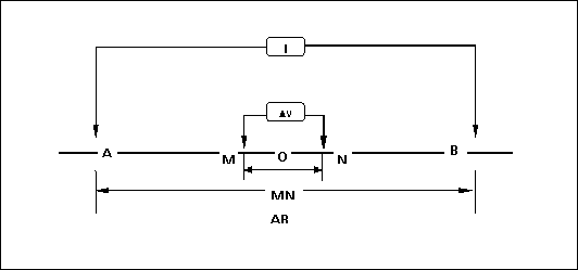
Schlumberger method is used most as a measuring system. In this method the electrodes are put in a line and point O is the common point between AB line and MN line. The AB/MN relationship is usually used in the greater Schlumberger method. Generally the results from the electrical soundages are offered in a way that ρa is the subordinate from the length of OA or AB/2 and the related diagram is drawn in the 2-logarithm coordinates system.
The appearing apparent resistivity is superficial concept and should not be attributed to as the medium resistivity in the underground heterogeneous constituents. In order to interpret the quantity of the appearing apparent resistivity we should consider the flow source points and the potential, because the amount of this quantity depends on the geometrical factor of the source points and the potential (Factor K).

2.1 Geo-electrical Resistivity Meter Devices
The electrical survey devices for measuring the electrical apparent resistivity are designed in a way that they measure the portion of ΔV/I in the equation (1) so precisely. Usually ΔV is counted by milli-volt and I by Milliamp in measurements. So we can calculate (K) by measuring these two appearing apparent resistivity parameters using the equation (1) and regarding the type of the electrodes order and its geometric factor.
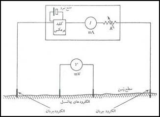
The apparent resistivity measurement devices consist of a direct current source (DC) or (AC), one milliamp meter and one milli-volt meter. Other equipments include the metal cables and electrodes which are installed into the ground as the AB electrodes and MN potential. The equipments used in the geophysical investigation operations for the subject of the study include a 10-500 voltage DC current producer with the current intensity of one ampere. The precision of the device in current intensity is 0.01 milliamps and 0.01 milli-volts for the voltage (Potential difference). In shape 2.2 the general principles of the structure of the apparent resistivity measurement device has been demonstrated.

2.2 WDDS-1 Electrical Resistivity Measurement Devices

General specifications of the device: -Automatic voltage measurement (-6 ~ +6 V)
-Automatic current measurement
-Ground productive potential control (SP) automatically (-1 ~ +1 V)
-The capability of saving more than 1200 off-takings.
-Automatic Hold capability of the measured current and voltage after injection time termination.
-Reset capability
-Internal battery charging capability.
-Adjustment of the output voltage from 10 to 700 volts.
-Maximum current output: 3.5 ampere
-Maximum power: 2450 w
-Approximate weight: 3 kg
-Ground apparent resistivity measurement (0/1kΩ ~ 200 kΩ)
-Functionality temperature: -10 to 60 centigrade.
-Measurement delay time: 0.1 to 5 seconds

Section Three: Interpretation Method for the Pseudo Sections and Resistivity Sections
As mentioned before, the geophysical off-takes are taken with a high density and in the electrical pseudo-section forms. The interpretations of the results have been performed in two qualitative and quantitative ways. In the qualitative interpretation it was tried that the measurements results be obtained without any interference or change. While in the quantitative measurements interpretation we tried to evaluate the apparent resistivity distribution of the subject of the survey using the mathematical models and processing the multi-layer continued models on the observed data.

3.1 Modeling the 2-Dimensional Resistivity Sections
The aim of this method has been driving the lateral vertical changes of the apparent resistivity with high density in the measurement points depending on the investigation depth. The basis of this method is that the more the distance is between the electrodes the deeper is transmitted electricity into the ground continuously. Thus the appearing apparent resistivity changes curves are provided on account of the subordinate of the electrode distance. By changing the orders of the four electrodes along the survey route we can easily both investigate the apparent resistivity changes in relation to the depth and investigate the apparent resistivity changes laterally. One of the precise methods for investigating the apparent resistivity in the underground environment is apparent resistivity 2-dimensional pseudo-sections methods with the high density measurement points. The precise model from the underground is a 2-dimensional model bearing the apparent resistivity changes both in range with the perpendicular and also in range with the side or horizon of the survey line.
This is supposed in this model that the apparent resistivity in range with the vertical line does not change on the survey route and is fixed. This presumption, apparently on the long geological masses, is acceptable to some extent and is a logical theory.
Nevertheless, the 2-dimensional survey of the apparent resistivity is the most economical geophysical survey method. In case of rejecting such assumption, the 3 dimensional surveys can offer more precise results, although many of them will be expensive. Today, one of the developed methods in geophysical engineering studies is the utilization of two dimensional electrical surveys with high density measurement points which is called the electrical tomography survey or electrical imaging. The difference between this method and the electrical soundage or profiling method is the number and density of the measurement points. This method is effective apparently in the geological complicated areas.

Modeling theory:

The way of converting used by this program is based on the smoothness constrained squares which is based on the following equation:

(J^TJ+uF)d=J^Tg

Where,

The beneficial point of this method is that the control factor and the smoothest filters can be adapted to various data. Please refer to gratitude succinct classes of Professor Loke (2001) for more details in respect to the smoothness constrained least squares various types.
This program supports a new compatibility based on the Quasi–Newton optimized technique in the least squares method. This technique is used for huge amount of data and is at least ten times faster than the common least squares method and requires less memory. The other way to perform this program is Quasi–Newton which is slower than Quasi–Newton but it offers a bit better results in the regions where the apparent resistivity amounts is 10 to 1. The third option in this program is using the Gauss-Newton for the second and third repetitions after Quasi-Newton method is used.
The two dimensional model used by this program divides the underground surface into some square blocks. The aim of this program is specifying the apparent resistivity of the square blocks in which ultimately the apparent resistivity attributed to these blocks provide a resistivity pseudo-section which is in compliance with the real measurement amounts. In the Wenner and Schlumberger orders, the first layer thicknesses of the blocks are 0.5 times less than the electrode distance. Fore the pole-pole, two pole and pole-two pole, this thickness is respectively 0.9, 0.3 and 0.6 times less than the electrode distances.
The thickness of the deeper layers generally increases 10% or 25%. Also, the user can change the depth of the layer manually.
This program basically tries to decrease the differences among the measured and calculated apparent resistivity amounts. The measurement of this difference is offered by root mean square error of the squares (RMS). Nevertheless, a model with the least error RMS in respect to the bigger and unreal changes in the model apparent resistivity is not necessarily and geologically the best model. In any general way, the best way of model choosing is choosing the model which does not repeat the RMS errors significantly. This usually occurs between 3 to 5 repeats.

3.2 Bi-Dimensional Electrical Surveys (Iso-Resistivity Pseudo-Sections)
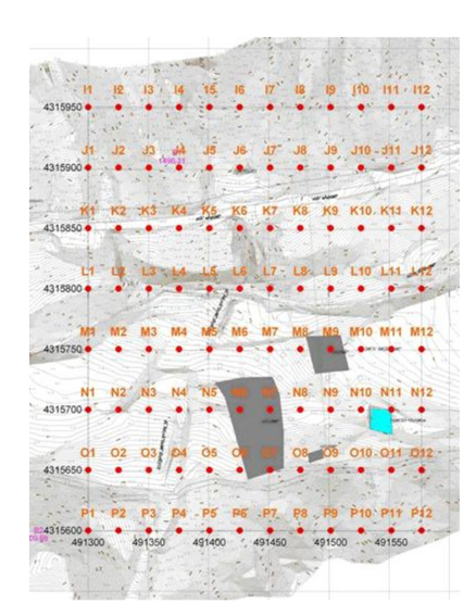
These investigations totally include 96 measurements which have been performed with the (V.E.S.) Schlumberger perpendicular method with the maximum current line length of 600 meters. In all of the offered appearing apparent same resistivity sections-like, the horizontal axis, the off-taken soundage places and the perpendicular axis equal to the half of the current line length (AB/2). In order to identify the geological structures and the type of the subject of study more precisely, the said sections-like have been investigated for the profiles in two ranges of north-south and west-east. Map1 shows the off-taken soundage in the area of the subject of the study. The position of each profile has been shown beside its iso-resistivity pseudo sections.

3.3 The Profiles Surveyed on the Western-Eastern Axis
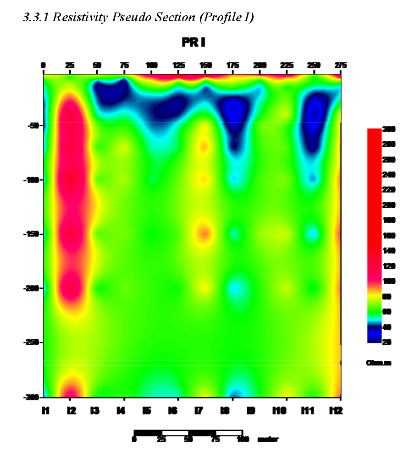
In the investigation region, 8 iso-resistivity pseudo-sections, related to the profiles in north east–south west ranges with the approximate soundage distances of 25m were investigated which are demonstrated in the following shape.

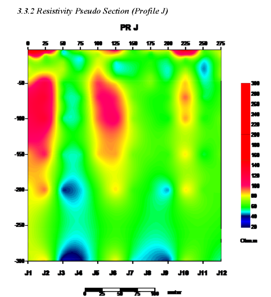
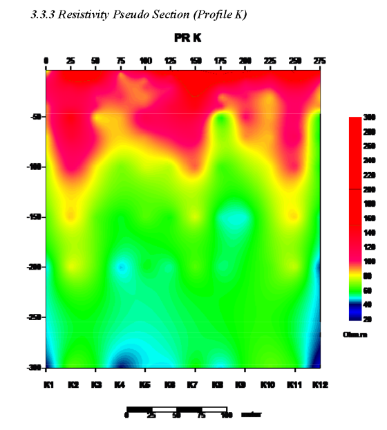
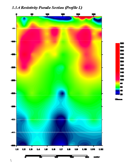
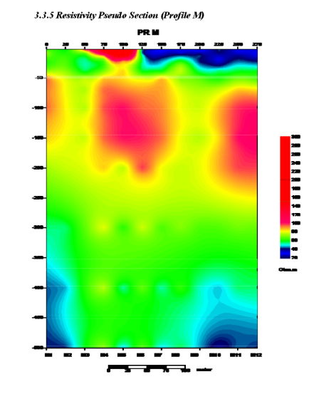
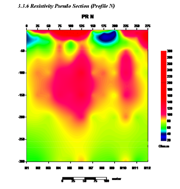
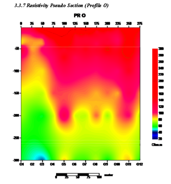
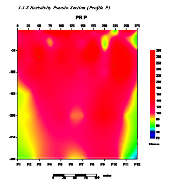
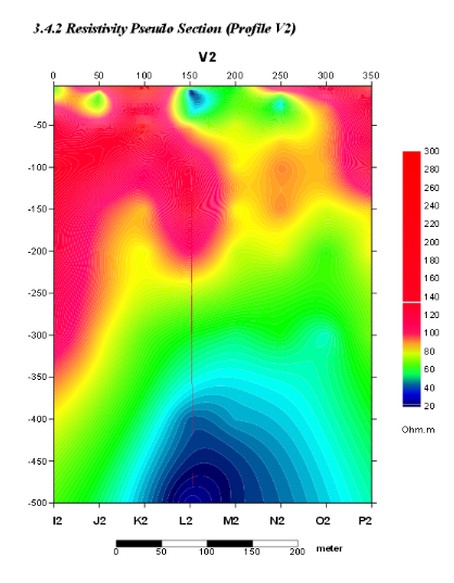
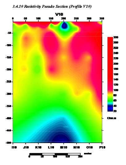
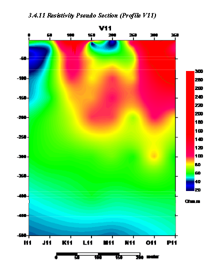
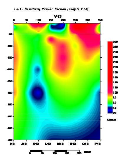
3.4 The Profiles Surveyed on the North-South Axis
In the investigation region, 12 iso-resistivity pseudo-sections, related to the profiles in north–south with the approximate soundage distances of 50m were investigated which are demonstrated in the following shape.

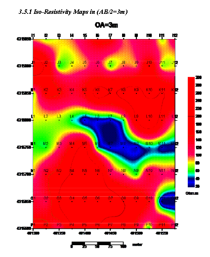
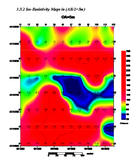
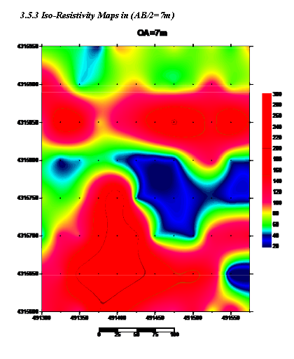
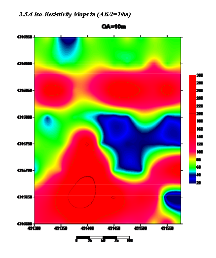
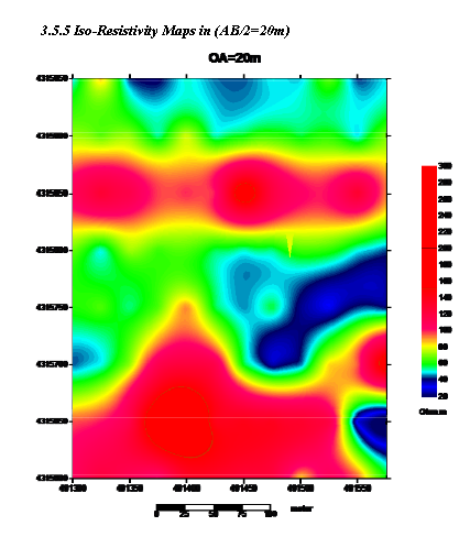
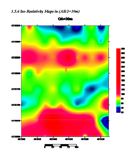
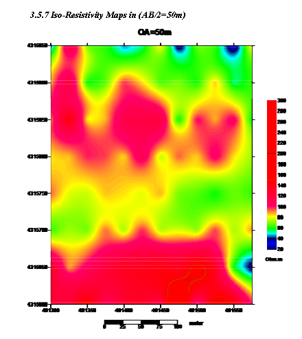
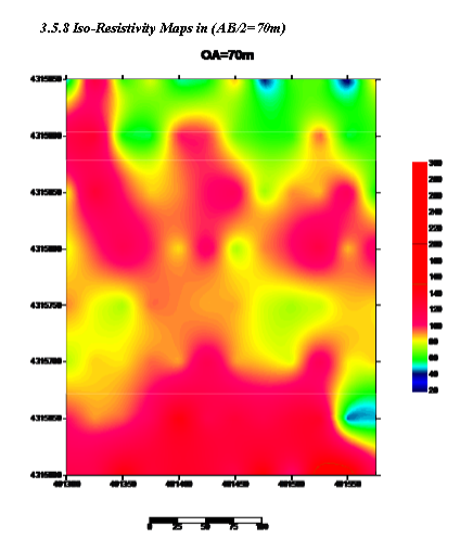
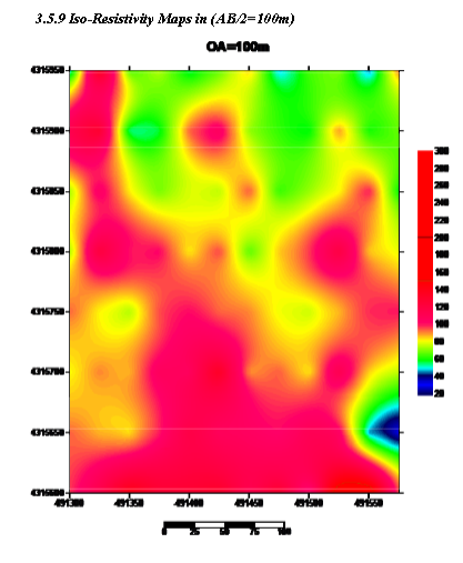
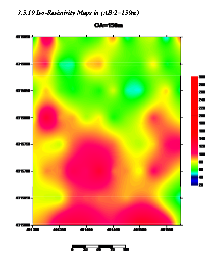
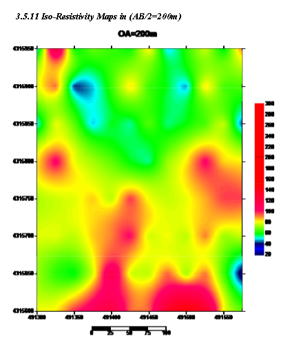
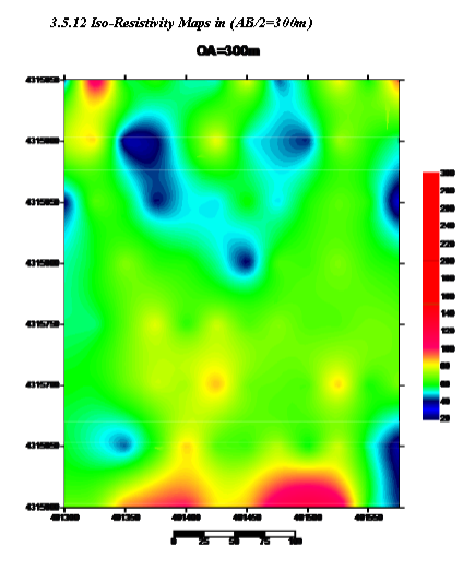
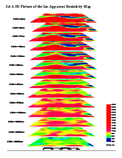
3.5 Iso-Resistivity Maps
In order to provide better images from the appearing apparent resistivity amounts in various depths, we have provided appearing apparent same resistivity maps for AB/2 (half of the length of the current line length). However we can not read depth and resistivity directly from the vector because the vectors resulted from the perpendicular electrical soundage do not demonstrate the apparent resistivity changes in relation to the length of the current electrodes. Thus these curves should be interpreted to obtain the depth of each electrode distance. The relation of these two depends on the thickness and electrical resistivity of the layers. In Iran the experiences show that AB/4 could be deemed as equal to the relation of depth and length of the current electrodes. In these studies, the appearing apparent same resistivity have been drawn for half of the length of the current lines of 3, 5, 7, 10, 20, 30, 50, 70, 150, 200, 300 meters each of which demonstrate the appearing apparent resistivity changes in the depth equal to half of the said current line length at the investigation region.

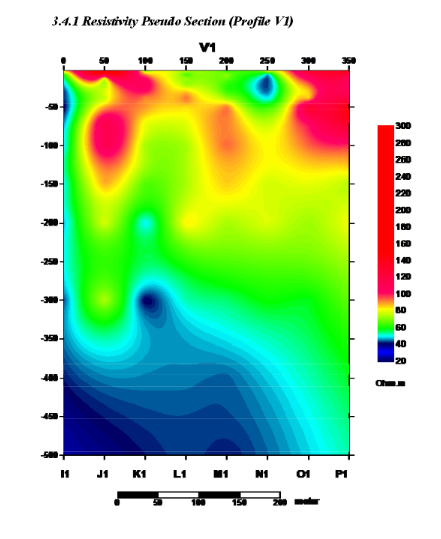
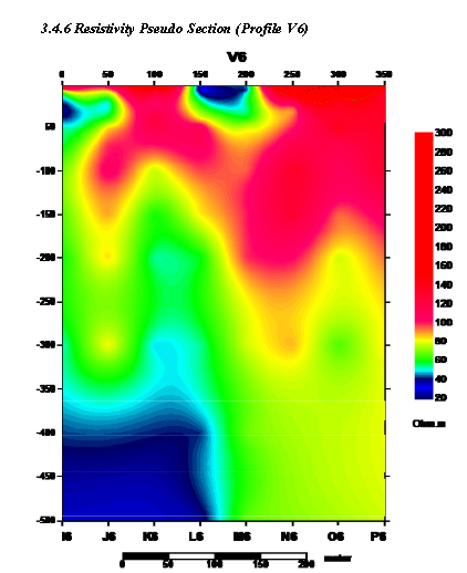
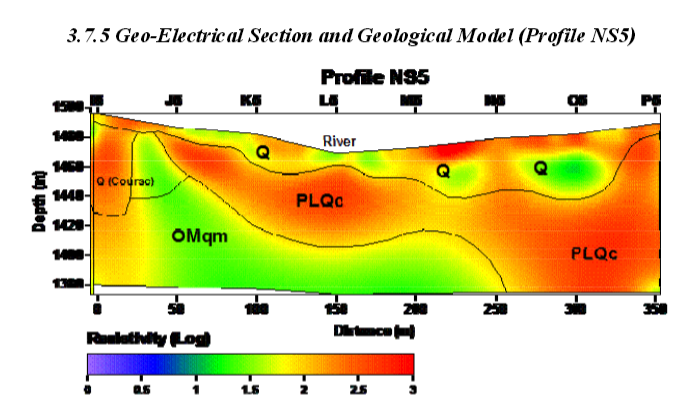
3.7 Modeling the Profiles Surveyed on the North-South Axis
Regarding the geological structure of the region and the fact that the related dam is located on an east-west axis river, the geo-electrical data modeling was performed on the vertical section on the main structure (North-South).
In all of the profiles we can segregate three existing lithologies in the region.
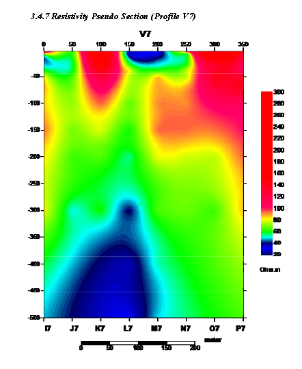
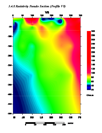
The quaternary deposits, conglomeratic Pleistocene and the upper surface of Ghom-formation which is made of marl. The general lithological changes trend of the region is as if the bed rock has stretched up its marl towards the north. In this trend towards the east the electrical conductivity of the Marl section of Ghom-formation is increased which demonstrates the increased amount of clay (Profiles 7 and 8).
According to the hydrogeological studies, the underground water surface of the region in Sabrkhan Village has been reported as 12 meters with respect to a well with the depth of 27 meters. In other wells of the region the water surface is less than 20 m. Therefore in the geoelectrical study region there is water saturation, thus there is no need to amend the Archie Law in the region.

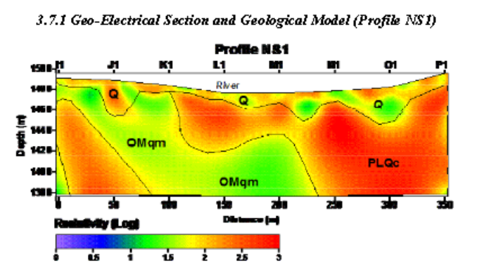
Three constituents of Conglomerate Pleistocene, marl of Ghom formation and the alluvium is separable in this region. The studied lithologies are shown respectively by PLQc, OMqm and Q.
The Conglomerate Pleistocene apparent resistivity is considered as higher than 100 ohm-meter. Due to the marl and clay inter-layers, the amount of this resistivity has been reduced. 10 to 100 ohm-meters are attributed to the upper section of Ghom formation. The thickness of the surface alluviums reach to maximum 30-40 depth which is changeable laterally. Fine grain deposits in the alluvium result in the less apparent resistivity and coarse grain deposits in the alluvium result in the higher apparent resistivity.

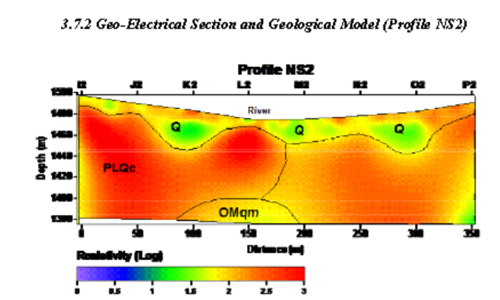
As shown in the picture, the depth of Marl in Ghom formation is increased in this section. The more we go to the south, the amount of conglomerate clay is increased which is shown as the decrease of the apparent resistivity. Comparing this section and the previous section, the lateral lithological change of the region is evident.

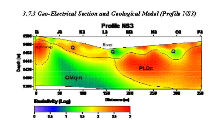
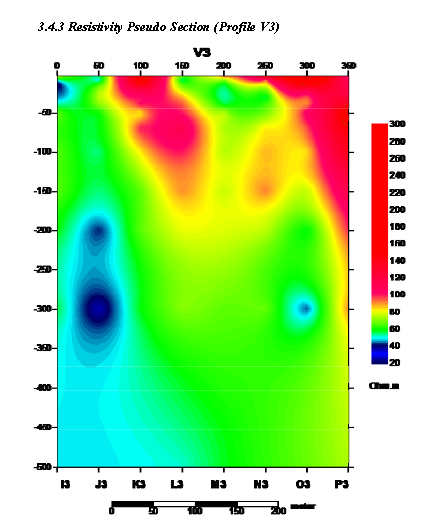
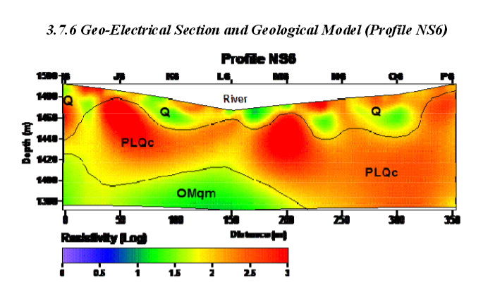
In this section, like the previous two sections, the alluvium layer is quite obviously segregated. However, in this section a large thickness from the coarse grain alluvium is demonstrated towards the north as in the form of “Coarse”. We see the lithological lateral change of respectively from marl to conglomerate from the north to the south in the distances of 170 m to 200 m on the profile. The amount of up-coming of the marl of bed rock is so high in this profile (up to 30 meters).

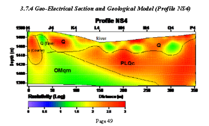
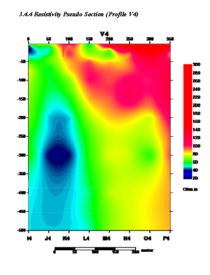
In this section the alluvium layer is separable too. The depth of the marl of bed rock is decreased in this section. The thickness of the conglomerate layer is increased towards the north. According to the geophysical evidences the amount of clay of the conglomerate layer is increased. In this section the coarse grain deposits are separable from the fine grain deposits towards the north.

In this section, the lithological changes are the same as the ones in section No. 4 however the alluvium thickness is decreased towards the north.

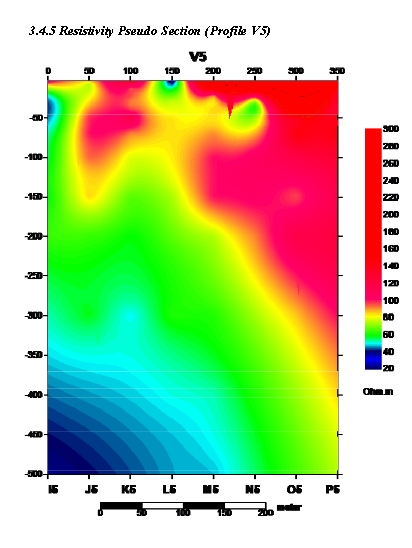
Regarding this section the stretching quality of the marl of bed rock inwards is completely evident. The conglomerate thickness is increased in this section. Moreover, the alluvium layer is noticeable like the previous section.

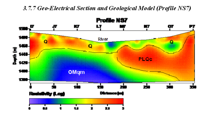
In this section, the clay amount of marl section of Ghom formation is increased which are demonstrated as the low apparent resistivity (Blue) amount. This issue is geotechnically significant regarding the fact that this is evident in soundage No. 8. We can see the lateral change of marl to conglomerate in approximately 180 meters. The common boundary between marl and conglomerate is continued from the 180 m to 330 m on the profile.

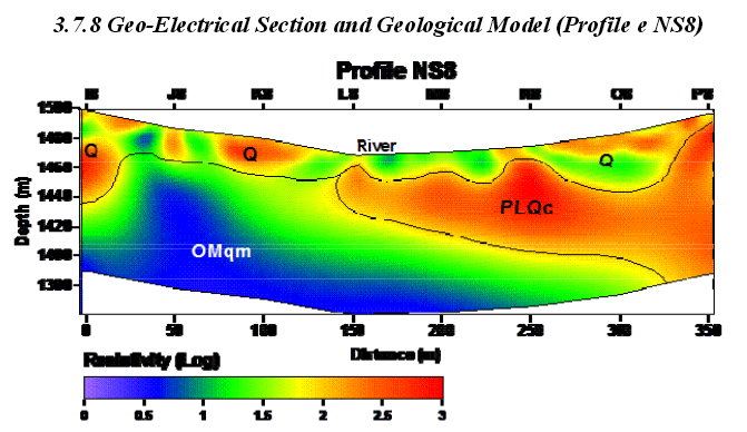
All of the cases mentioned in section No. 7 is evident in this section too but the conglomerate is drawn and stretched thinner towards the north and the marl of bed rock is brought onto upper sides.

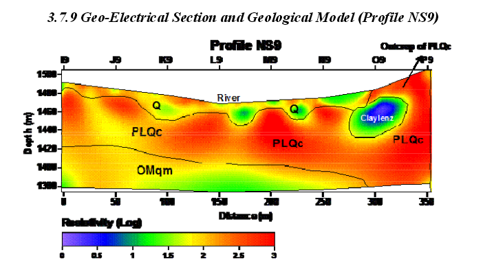
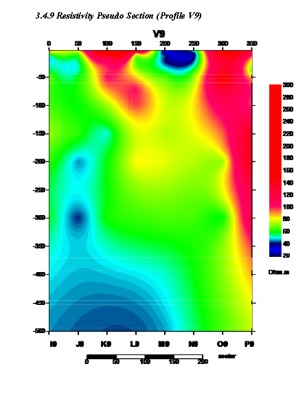
The conglomerate layer has covered all the section towards the north and the depth of the marl of bed rock is increased. Generally, in this section and other sections, the changes between Ghom formation and conglomerate are so gradual. Conglomerate emerging in the south end of the section is noticeable. Also, a clay lens mass is noticeable in 300 m distance.

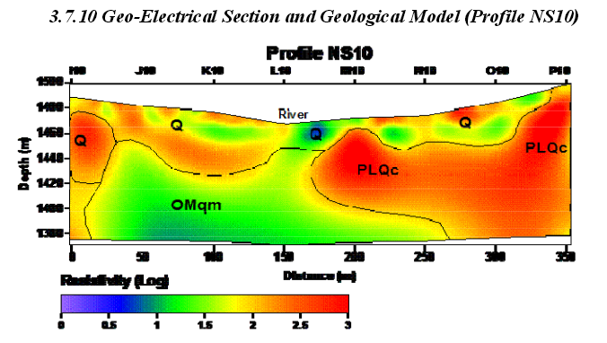
The lateral changes of this region are evident regarding the various sections. The lateral changes between this section and section No. 9 is completely evident in 25-m distance. In this section, the bed rock has lifted up its marl. The conglomerate is emerged in the south end of the section.

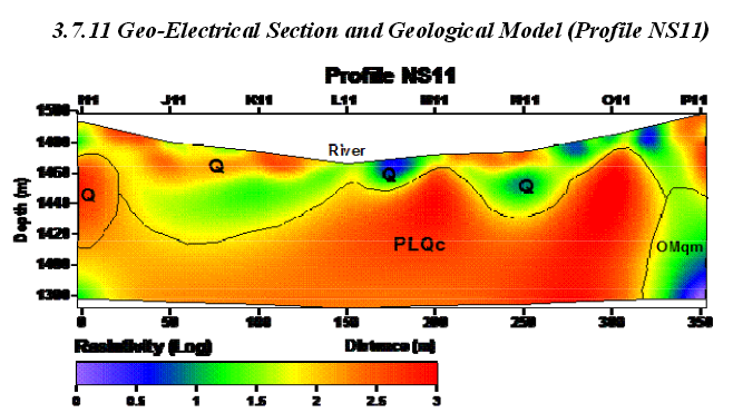
Again in this section the marl of the bed rock is stretched up.

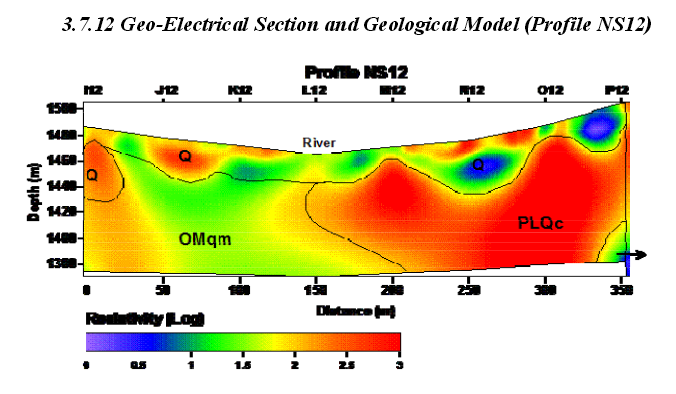
This section is the same as the structure of the section No. 10

3.8 Conclusion and Recommendations

Discussion:

According to the interpretations of the geophysical sections discussed in details in previous section we can lithologically segregate three layers. The first layer is alluvium in which according to its appearing apparent resistivity we can separate the coarse grain (High resistivity) and fine grain (Low resistivity) sections from each others. The thickness of alluvium is different in northern sections from southern ones changing from 10 to 50 meters. Another significant issue which is evident in the layer beneath the alluvium (conglomerate) is the lateral changes of this layer apparently in the east-west range. Regarding the seeming issue that the conglomerate layer changes are due to the uplifting of the pull-down of the bed rock, marl has been created. The required measures should be taken in this regard in order to make a dam. As mentioned before, the 3rd layer is Marl Ghom formation Rock. The changes from profiles L and M in most sections from Ghom formation to conglomerate is quite gradual and only the appearing changes are evident. Therefore clefts are not much likely to be created.
In profiles 7 and 8 the low resistivity of Marl of bed rock proves the existence high amount of clay which should be considered in dam construction in respect to the lack of tension capability in infrastructures.

Recommendations:
It seems that the geophysical studies is well performed by geoelectrical method in the region and has determined the geological ambiguities concerned by the geologist engineers.
Regarding the fact that the geotechnical trial holes possibility in the region is definite, preferably at least 2 trial holes between L7 and M7 points in Ns7 section and also between L8 and M8 in Ns8 section should be drilled.
Furthermore, it is suggested to use in-well quake method, as a cheap and effective method in obtaining the earth dynamic parameters, apparently in two mentioned boreholes and also in other boreholes suggested by the geologist engineers.